The Frequency Response of Mathieu's Equation

Karthik Chikmagalur

Motivation
Modelling time-periodic systems
Lifting
Numerical Solution through Discretization and Lifting
Poles of the lifted system
Singular values of the lifted system
Characterizing the free response
The \(H_2\) norm of Mathieu's Equation
Conclusions
Ongoing and future work
References

Motivation

Time-periodic dynamical systems

Three related ideas

Parametric Excitation

Excitation of oscillations through parametric forcing

Parametric Resonance

Destabilization of system response through parametric forcing

Vibrational Stabilization

Parametric stabilization of nominally unstable system behavior

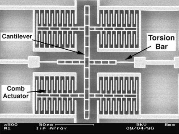
Microcantilever based mass sensing

[turner1998]

\[I \ddot{\theta} + c \dot{\theta} + k \theta = M(t,\theta) \]

MEMS devices used as capacitive sensors can operate at high frequencies, with high sensitivities and low power requirements.

Can utilize parametric excitation to decouple sensitivity from bandwidth (Q factor)

Capacitive sensing is also sensitive to parasitic signals from the actuating drive signal.

Parametric Excitation

Can achieve very high Q factors not currently attainable with present resonance mode AFM techniques.

Control of Stirling engines

[craun2015]

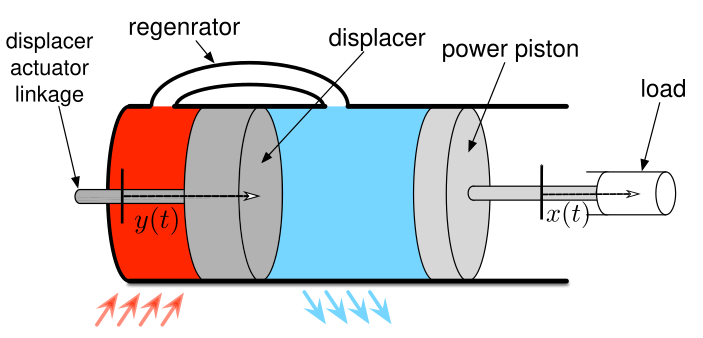
The simplest dynamical model of a Stirling engine is the Schmidt model:

\[\ddot{x} + c \dot{x} + \frac{x-y}{1+x-y} = 0\]

Which exhibits parametric resonance for certain periodic displacer motions \(y(t)\).

When linearized about \(x = 0\), with \(y(t) = \epsilon \cos(\omega t)\),

\(\ddot{x} + c \dot{x} + (1+2 \epsilon \cos(\omega t)) x = 0\)

Parametric Resonance

Instability in the system as a result of parametric variation

Vibrational stabilization

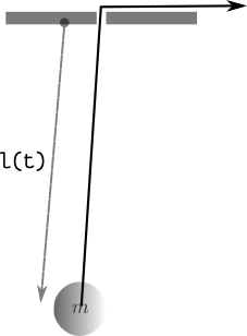
A rigid pendulum where the pivot point oscillates in the vertical direction.

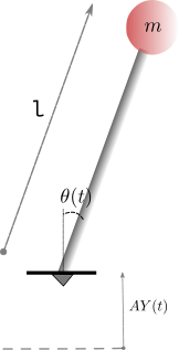
\[\ddot{\theta} + \left( -\frac{A}{l}\ddot{Y}(t) - \frac{g}{l} \right)\sin(\theta) = 0\]

Vibrational Stabilization

The Kapitza pendulum can be vibrationally stabilized with the right pivot motion \(AY(t)\).

Parametric Resonance in Mechanics

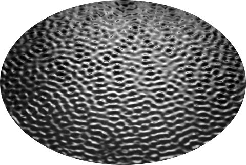
Linear stability of Faraday waves when a container is oscillated vertically [benjamin1954]

Kelvin-Helmholtz instability with time-periodic shear [kelly1965]

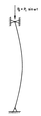
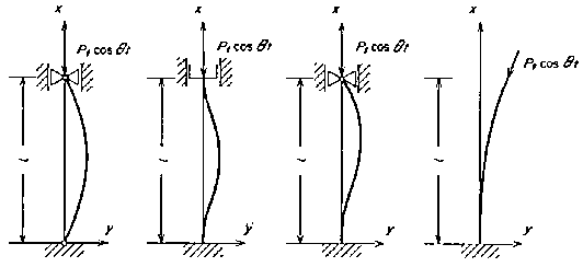Vibrations of columns subjected to oscillating axial loads [iwatsubo1974]

Parametric Resonance in Fluid Mechanics: More examples

Acoustic instabilities in flames [sammarco1997] and in Rayleigh-Bénard convection [vittori1998]

Stability of Barotropic and Baroclinic shear flows [poulin2003] and [pedlosky2003]

Modelling time-periodic systems

Mathieu's Equation

The canonical example of a periodic linear system is Mathieu's Equation,

\[\ddot{x}(t) + (\pm \omega^2 + \epsilon \cos{t}) x(t) = 0\]

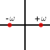
\(+\omega^2\): Is a harmonic oscillator with a periodically time-varying spring constant

\(-\omega^2\): Exponentially unstable in the absence of parametric forcing, corresponds to a system like the Kapitza pendulum.

Mathieu's Equation with viscous damping

\[ \ddot{x}(t) + 2 \nu \omega \dot{x}(t) + (\pm \omega^2 + \epsilon \cos{t}) x(t) = 0 \]

Can be transformed through a change of coordinates \(\bar{x} = x(t) e^{\nu \omega t}\) to Mathieu's Equation

The Hill ODE

Mathieu's Equation is a special case of the more general Hill ODE

\[\ddot{x}(t) + f(t) x(t) = 0 \text{, }f(t+T) = f(t)\]

where \(f\) has a single harmonic.

\[x(t) = \Phi(t,t_0) x(t_0)\]

The Hill ODE is formally solved using Floquet theory: Its stability is determined by the eigenvalues of the Monodromy map \(\lambda[\Phi(T,0)]\), where \(\Phi(t,t_0)\) is the state transition matrix.

The Hill ODE is measure preserving, \(\frac{d}{dt} \det \Phi(t,s) = 0\)

Measure preserving

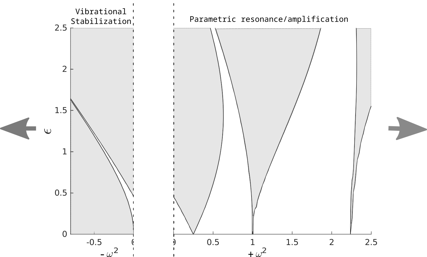
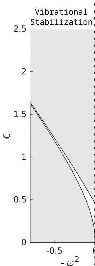
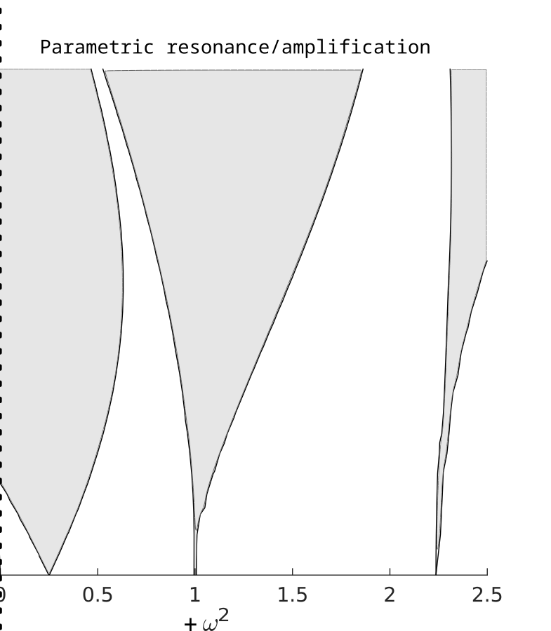
\begin{align*} \frac{d}{dt} \det \Phi &= \det \Phi\ Tr \left[ \dot{\Phi} \Phi^{-1}\right]\\ &= \det \Phi\ Tr \left[ \left( \begin{smallmatrix} 0 & 1\\ \star & 0\end{smallmatrix}\right) \Phi \Phi^{-1} \right]\\ &= \det \Phi\ Tr \left[\left( \begin{smallmatrix} 0 & 1\\ \star & 0\end{smallmatrix}\right) \right] = 0 \end{align*}

Mathieu's Equation: Stability

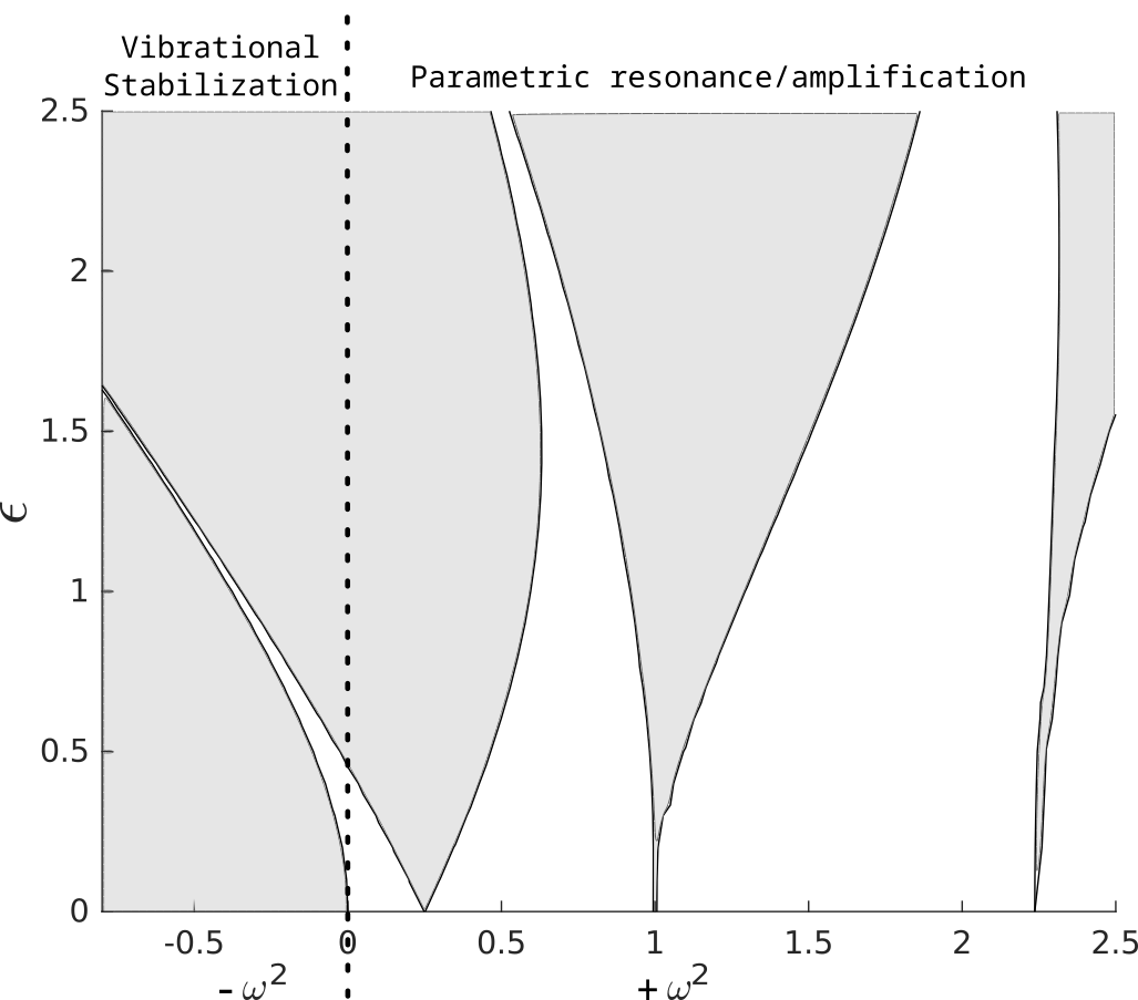\[\ddot{x}(t) + (\pm \omega^2 + \epsilon \cos{t}) x(t) = 0\]

Parametric Amplification or Resonance

\(+\omega^2\): A nominally stable (\(\epsilon = 0\)) harmonic oscillator can be destabilized with parametric forcing of very low amplitude if the forcing frequency is chosen carefully.

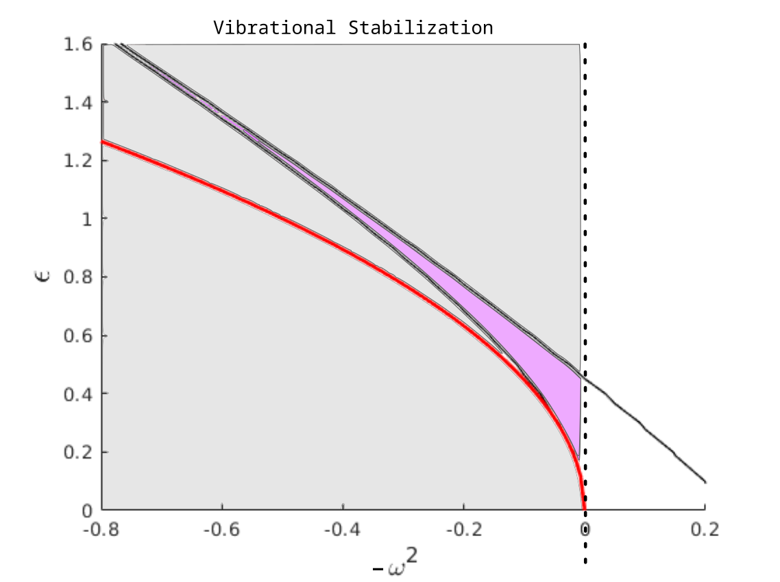
Vibrational Stabilization

\(-\omega^2\): The right combination of \(\epsilon\) and forcing frequency can stabilize the system.

Vibrational stabilization - Averaging

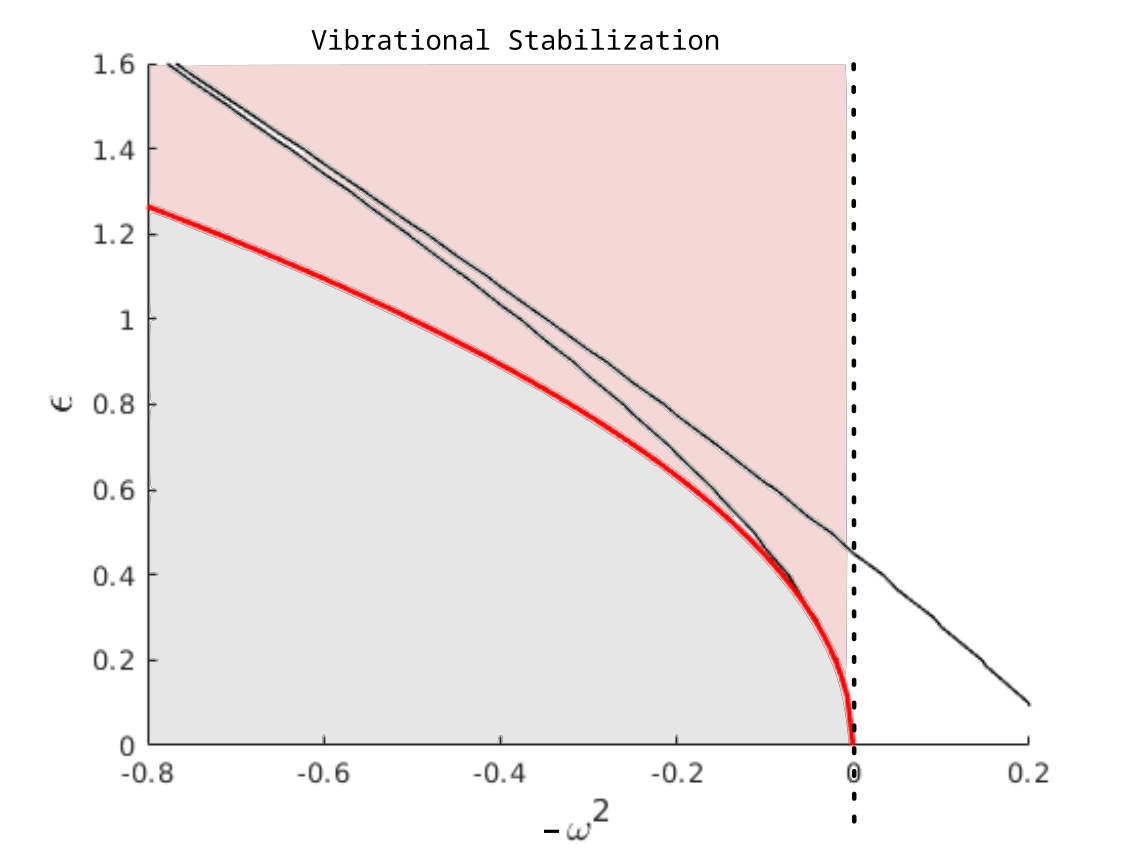
\[ \ddot{x}(t) + (- \omega^2 + \epsilon \cos{t}) x(t) = 0 \]

Averaging methods relate the stability of a time varying system \(\dot{x} = f(t/\alpha, x)\) to that of a time-invariant averaged system \(\dot{x} = F(x)\) as \(\alpha \rightarrow 0\).

[Berg_2015]

For Mathieu's Equation:

For \(\epsilon^2 > 2 \omega^2\), \(\exists\) \(\omega^{\star}\) such that the origin is (Lyapunov) stable for \(\omega < \omega^{\star}\)

Questions of Interest

Given a viable range of parameters \((\omega,\epsilon)\), how do they differ in performance?

How sensitive are different possible operating points of a parametric amplifier to noise?

How robust is the vibrationally stabilized region of parameter space to disturbances?

Addressing these questions requires understanding the input-output characteristics of the system

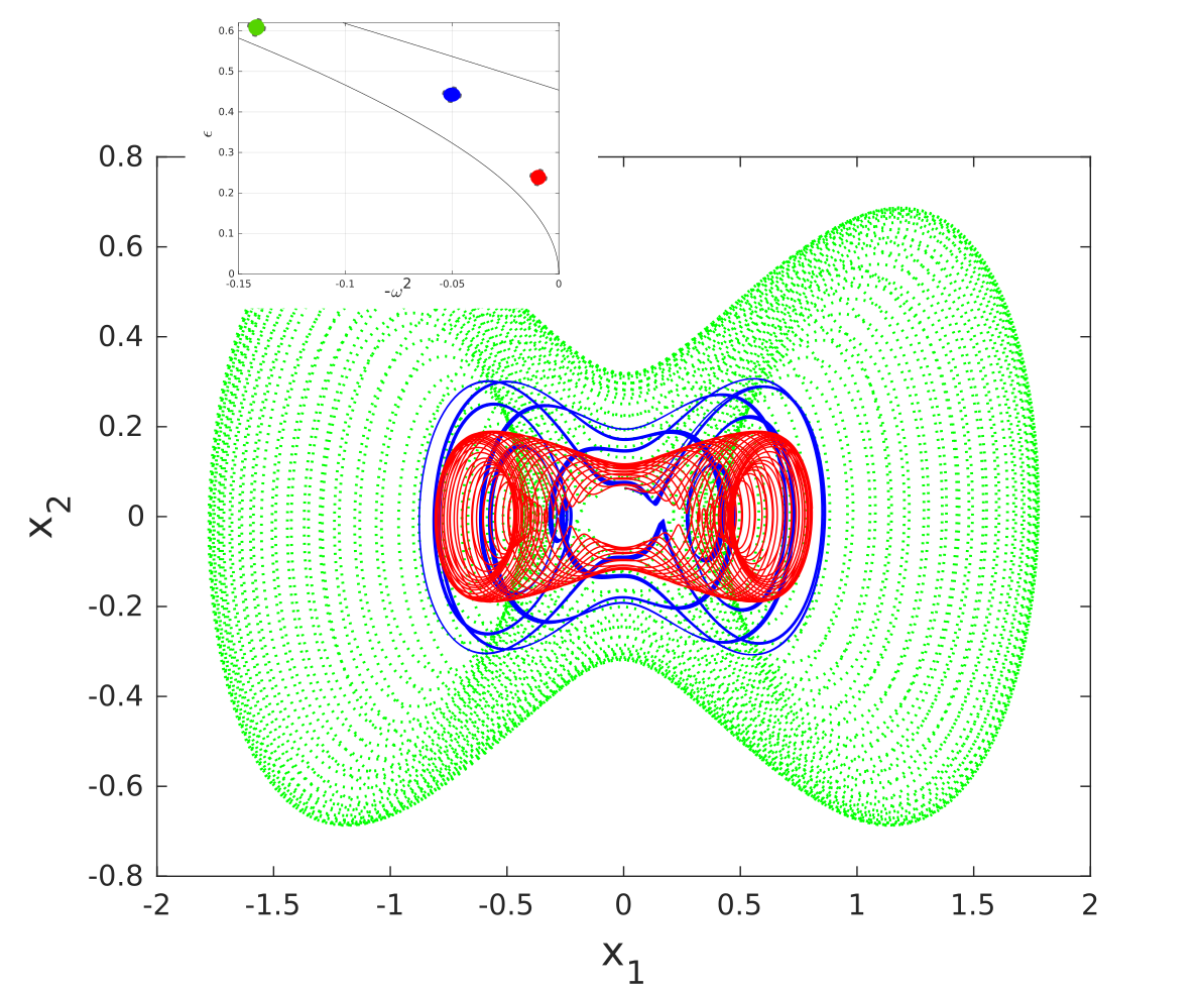
Impulse response at different operating points

\[\ddot{x}(t) + (\pm \omega^2 + \epsilon \cos{t}) x(t) = \delta(t)\]

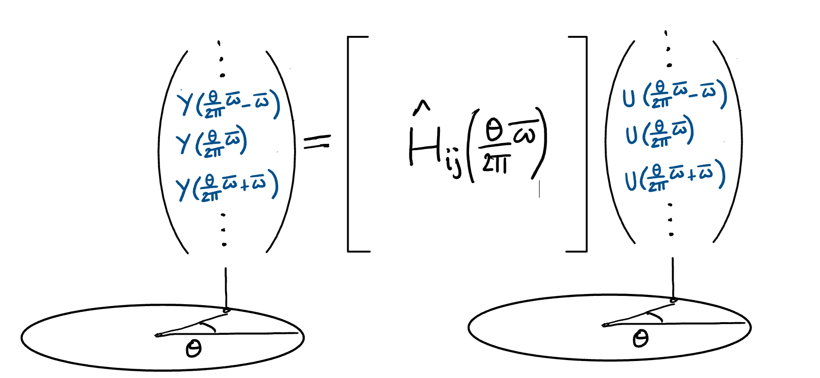
Input-Output characteristics

"Transfer function" analysis: Let \(\bar{\omega} = \frac{2\pi}{T}\). Then

\begin{equation} \underbrace{\begin{bmatrix} \vdots\\ X(\omega-\bar{\omega})\\ X(\omega)\\ X(\omega+\bar{\omega})\\ \vdots \end{bmatrix}}_{\hat{X}(\omega)} = \underbrace{\begin{bmatrix} & & & & \\ & & & & \\ & &\hat{H}_{ij}(\omega) & & \\ & & & & \\ & & & & \\ \end{bmatrix}}_{\hat{H}(\omega)} \underbrace{\begin{bmatrix} \vdots\\ W(\omega-\bar{\omega})\\ W(\omega)\\ W(\omega+\bar{\omega})\\ \vdots \end{bmatrix}}_{\hat{W}(\omega)} \end{equation}

Lifting

Lifting allows us to represent a time-periodic system as a time invariant one in a space with higher dimensional input and output spaces

Representing periodic systems as LTI

CONTINUOUS TIME, PERIODIC

\begin{align*} G: \begin{cases} \dot{x}(t) =& A(t) x(t) + B u(t)\\ y(t) =& C u(t) \end{cases} \end{align*}

where \(x(t) \in \mathbb{R}^n\), \(u(t) \in \mathbb{R}^p\), \(y(t) \in \mathbb{R}^m\).

DISCRETE TIME, LTI

\begin{align*} \hat{G}: \begin{cases} \hat{x}_{k+1} =& \hat{A} \hat{x}_k + \hat{B} \hat{u}_k\\ \hat{y}_{k} =& \hat{C} \hat{x}_k + \hat{D} \hat{u}_k \end{cases} \end{align*}

where \(\hat{x}_k \in \mathbb{R}^n\), \(\hat{u}_k \in L_2^p[0,T]\), \(\hat{v}_k \in L_2^m[0,T]\).

Lifting of Signals

\(f \in L_{N,e}^p[0,\infty)\), \(1 \le p < \infty\): Extended space of continuous time \(N\) -vector signals

\(\hat{f} \in l^p_{L^p[0,T]}\): Space of sequences which take values in \(L^p[0,T]\).

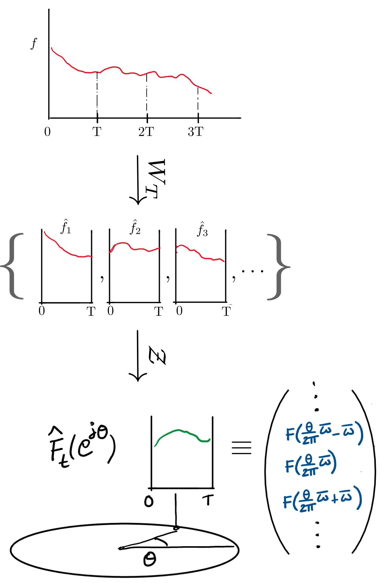
The lifting operator \(W_T: L^p[0,\infty) \rightarrow l^p_{L^p[0,T]}\), such that

\[\hat{f} = W_T f,\ \hat{f}_i(t) = f(T i + t),\ 0 \le t \le T\]

\(W_T\) breaks up the signal \(f\) into an infinite number of pieces, each of which is a shifted copy of \(f\) restricted to an interval \([0,T]\).

[bamieh1992h2]

Lifting of Systems

Let \(D_T\) and \(S\) be delay and shift operators:

\begin{align} D_T&:L^p \rightarrow L^p & (D_Tf)(t):=f(t-T)\\ S&:l^p \rightarrow l^p & S([x_0,x_1,\dots]) = [0,x_0,x_1,\dots] \end{align}

Then \(W_T D_T = S W_T\)

For any linear operator \(G: L^p[0,\infty) \rightarrow L^p[0,\infty)\), define its lifting as \[ \hat{G} := W_T G W_T^{-1},\ \hat{G}:l^p_{L^p[0,T]}\rightarrow l^p_{L^p[0,T]} \]

If \(G\) is \(T\) -periodic, then it commutes with the delay operator \(D_T\), \(G D_T = D_T G\)

Then \(\hat{G}S = S \hat{G}\), so \(\hat{G}\) is shift-invariant (LTI)

Representing periodic systems as LTI

CONTINUOUS TIME, PERIODIC

\begin{align*} G: \begin{cases} \dot{x}(t) =& A(t) x(t) + B u(t)\\ y(t) =& C u(t) \end{cases} \end{align*}

where \(x(t) \in \mathbb{R}^n\), \(u(t) \in \mathbb{R}^p\), \(y(t) \in \mathbb{R}^m\).

DISCRETE TIME, LTI

\begin{align*} \hat{G}: \begin{cases} \hat{x}_{k+1} =& \hat{A} \hat{x}_k + \hat{B} \hat{u}_k\\ \hat{y}_{k} =& \hat{C} \hat{x}_k + \hat{D} \hat{u}_k \end{cases} \end{align*}

where \(\hat{x}_k \in \mathbb{R}^n\), \(\hat{u}_k \in L_2^p[0,T]\), \(\hat{v}_k \in L_2^m[0,T]\).

\begin{align*} \hat{A}:& \mathrm{R}^n \rightarrow \mathrm{R}^n & \hat{A} \hat{x}_k =& \Phi(T,0) \hat{x}_k\\ \hat{B}:& \mathrm{L}_2^p[0,T] \rightarrow \mathrm{R}^n & \hat{B} \hat{u}_k =& \int_0^T \Phi(T,s) B \hat{u}_k(s) \mathrm{d}s\\ \hat{C}:& \mathrm{R}^n \rightarrow \mathrm{L}_2^m[0,T] & \left[\hat{C} \hat{x}_k\right](t) =& C \Phi(t,0) \hat{x}_k\\ \hat{D}:& \mathrm{L}_2^p[0,T] \rightarrow \mathrm{L}_2^m[0,T] & \left[ \hat{D} \hat{u}_k \right](t) =& \int_0^t C \Phi(t,s) B \hat{u}_k(s) \mathrm{d}s \end{align*}

Solution in terms of \(\hat{G}\)

\(\hat{G}\) is shift-invariant (in \(k\)) and so has a simple solution: \[\hat{y}_k = \sum_{j=0}^{k-1} \hat{C} \hat{A}^{k-j-1} \hat{B} \hat{w}_j + \hat{D} \hat{w}_k \]

\(\hat{G}\) has the semi-infinite Toeplitz representation \[\hat{G} \equiv \begin{bmatrix} \hat{D} & 0 & 0 & 0 & \dots\\ \hat{C}\hat{B} & \hat{D} & 0 & 0 & \dots\\ \hat{C} \hat{A} \hat{B} & \hat{C}\hat{B} & \hat{D} & 0 & \dots\\ \hat{C} \hat{A}^2 \hat{B} & \hat{C} \hat{A} \hat{B} & \hat{C}\hat{B} & \hat{D} & \dots\\ \vdots & \ddots & \ddots & \ddots & \ddots\\ \end{bmatrix} \]

Relating the Lifting operator to the Harmonic transfer operator

\begin{equation*} f(t) \overset{\text{Lift}}{\longrightarrow} \{ \hat{f}_k(\tau) \} \overset{\mathbb{Z}}{\longrightarrow} \hat{F}_t(e^{j \theta}) \overset{\text{Basis}}{\longrightarrow} \begin{bmatrix} \vdots\\F(\frac{\theta}{2\pi}\bar{\omega} - \bar{\omega})\\F(\frac{\theta}{2\pi}\bar{\omega})\\F(\frac{\theta}{2\pi}\bar{\omega} + \bar{\omega})\\\vdots \end{bmatrix}\\ \end{equation*}

Numerical Solution through Discretization and Lifting

Discretizing the Hill ODE

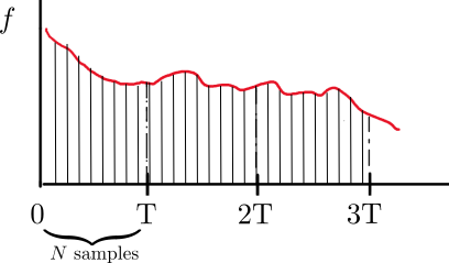
\begin{align} \dot{x}(t) &= \begin{pmatrix} \dot{x}_{1}\\ \dot{x}_2 \end{pmatrix} = \begin{bmatrix} 0 & x_1\\ -f(t) & 1 \end{bmatrix} x(t) + \begin{bmatrix} 0\\1 \end{bmatrix} w(t)\\ y(t) &= \begin{bmatrix} 1 & 0 \end{bmatrix} x(t) \end{align}

Discretized symplectically with \(N\) steps over period \(T\), then lifted

Method details

First order Euler backward/forward for the two components:

\(x_n = x(n \Delta),\quad f_n = f(n \Delta)\)

\begin{align*} x_{k+1} =& \begin{bmatrix} 1 - f_k \Delta^2 & \Delta\\ -f_k \Delta & 1 \end{bmatrix} x_k + \begin{bmatrix} \Delta^2\\ \Delta \end{bmatrix} w_k \label{eq:discretized-system}\\ =& \phi_k x_k + \beta w_k\\ y_k =& \begin{bmatrix}1 & 0 \end{bmatrix} \begin{bmatrix} x_{1,k}\\x_{2,k} \end{bmatrix} = \zeta x_k \end{align*}

Symplectic:

\(\phi_k^T \left( \begin{smallmatrix} 0 & 1\\ -1 & 0\end{smallmatrix} \right)\phi_k = \left( \begin{smallmatrix} 0 & 1\\ -1 & 0\end{smallmatrix} \right)\)

\begin{align*} \hat{x}(l) = x_{lN} &\quad \hat{w}(l) = \begin{bmatrix} w_{l N}\\w_{l N+1}\\w_{l N+2}\\\vdots\\w_{l N+N-1} \end{bmatrix} & \hat{y}(l) = \begin{bmatrix} y_{l N}\\y_{l N+1}\\y_{l N+2}\\\vdots\\y_{l N+N-1} \end{bmatrix} \end{align*}

Poles of the lifted system

Found as the eigenvalues of the Monodromy map \(\hat{A} = \Phi(T,0)\)

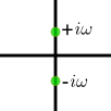
The Eigenvalues are constrained to the unit circle (when the system is stable) or the real axis (when unstable).

Since \(\Phi(0,0) = I\), \(\det \Phi(t,0) = 1 \forall t>0\)

\(\lambda_1 = \frac{1}{\lambda_2}\) and

\(\lambda_1^{\star} = \lambda_2\) or \(\lambda_1, \lambda_2 \in \mathbb{R}\)

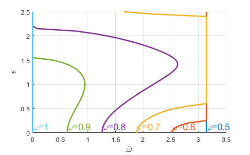
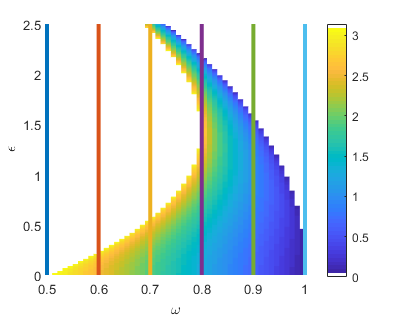
Eigenvalues of the Monodromy map

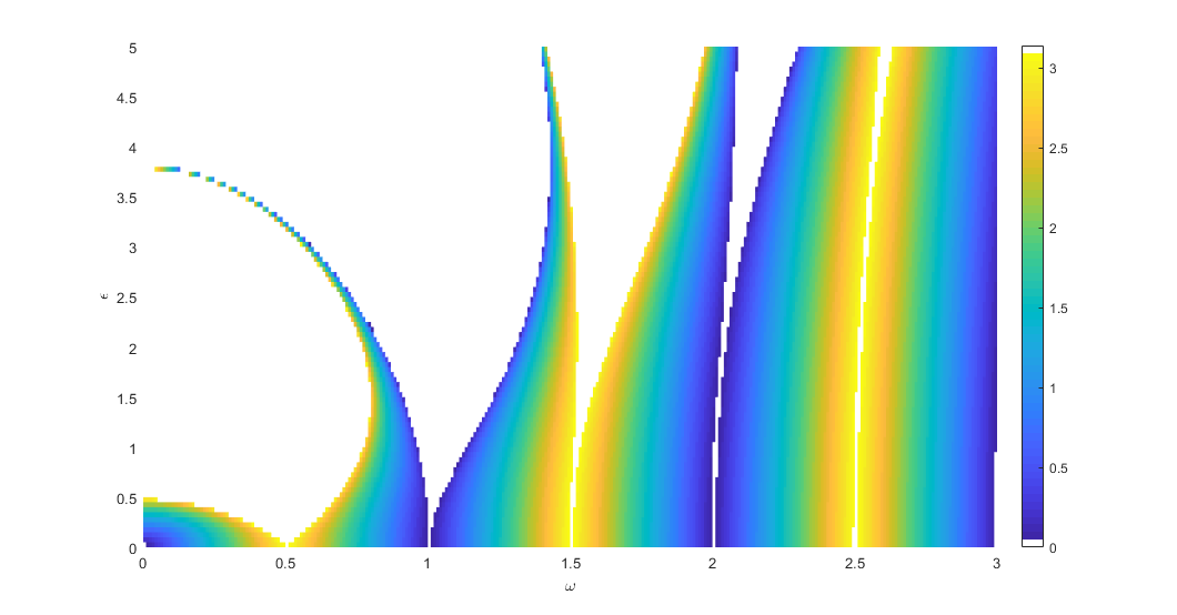
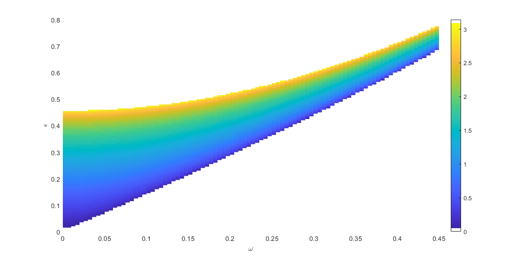
The argument of the eigenvalues is always \(0\) or \(\pi\) at the stability boundaries. In the stable regions the poles are \(e^{\pm j \bar{\omega}}\), \(0 \le \bar{\omega} \le \pi\).

discrete-mathieu-eigenvalues-stable-varying-epsilon.png

Singular values of the lifted system

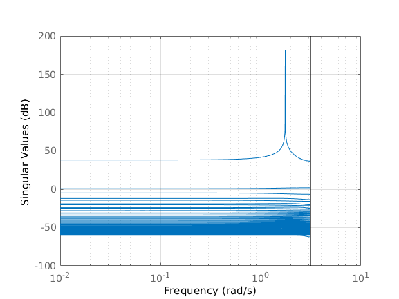
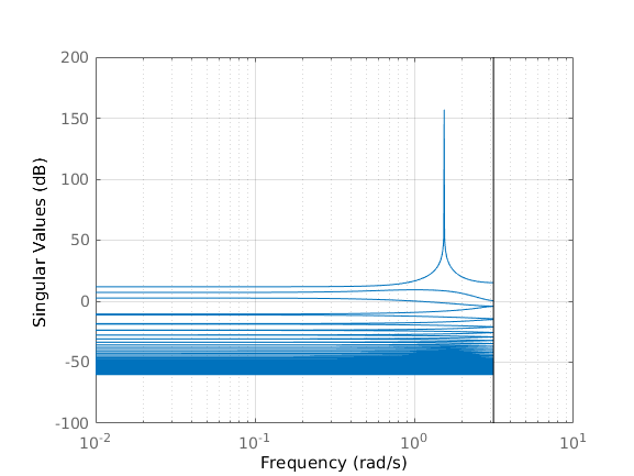
The lifted system has a single mode that grows at resonance. This suggests that its frequency response close to resonance is similar to that of a second order system.

Characterizing the free response

Transfer function of \(\hat{G}\):

\( \hat{G}(z) = \underbrace{\hat{C} (z I - \hat{A})^{-1} \hat{B}}_{\text{rank } 2} + \underbrace{\hat{D}}_{\infty \text{ rank but finite and bounded}} \)

Near resonance, \((z I - \hat{A})^{-1}\) is near-singular and outstrips \(\hat{D}\) in magnitude, so it depends on \(z\) through factors \((z - e^{\pm j \bar{\omega}})^{-1}\):

\[\hat{Y}(z) \approx \frac{c \hat{u}_1(e^{j \bar{\omega}})}{z - e^{j \bar{\omega}}} + \frac{c^{\star} \hat{u}_1(e^{-j \bar{\omega}})}{z - e^{-j \bar{\omega}}} \]

\(\hat{u}_1(e^{j \bar{\omega}})\): First left singular vector at resonance

Characterizing the free response

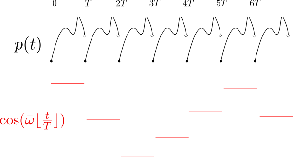
\(y(t) = p(t) \exp{\left(j \bar{\omega} \lfloor \frac{t}{T} \rfloor \right)},\ p(t+T) = p(t)\)

If \(\bar{\omega}\) is rational: periodic function, otherwise "almost periodic"

\(y(t) \stackrel{W_T}{\rightarrow} \hat{y}_k = p e^{j \bar{\omega} k}\)

\(\hat{y}_l = p e^{j \bar{\omega} (l-1)} \Leftrightarrow \hat{Y}(z) = \frac{p}{z - e^{j \bar{\omega}}}\)

\[\hat{Y}(z) \approx \frac{c \hat{u}_1(e^{j \bar{\omega}})}{z - e^{j \bar{\omega}}} + \frac{c^{\star} \hat{u}_1(e^{-j \bar{\omega}})}{z - e^{-j \bar{\omega}}} \Leftrightarrow y(t) \approx \Re \left[ c\ \hat{u}_{1,t}(e^{j \bar{\omega}})\ \exp \left\{j \bar{\omega} \left( \lfloor \frac{t}{T} \rfloor - 1 \right)\right\}\right] \]

The free response of Mathieu's Equation can be characterized as the product of copies of a "constant" function \(\hat{u}_1(e^{j \bar{\omega}})\) and an "almost periodic" complex exponential.

Free response vs first LSV of \(\hat{G}\)

Impulse response (full numerical solution)

Low rank approximation (using first LSV)

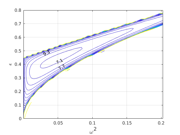
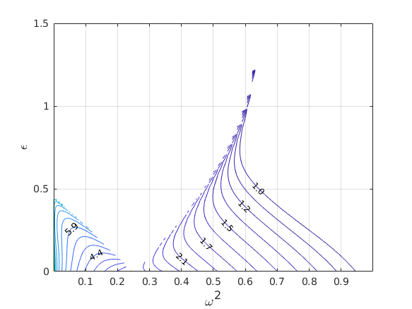
The \(H_2\) norm of Mathieu's Equation

The \(H_2\) norm is a measure of the system's input-amplification \[\left\lVert{G}\right\rVert_{H_2}^2 := Tr \left( \int_0^{\infty} G(t) G^{\star}(t) \mathrm{d}t \right)\] Square average of the norms of the responses to a set of unit inputs that excite all "parts" of the system.

The \(H_2\) norm of Mathieu's Equation

When \(G\) is \(T\) -periodic,

\[ \left\lVert{G}\right\rVert_{H_2}^2 := \frac{1}{T} \int_0^T Tr \left( \int_0^{\infty} G(t,s)G^{\star}(t,s) \mathrm{d}s \right) \mathrm{d}t \]

Collects contributions from impulses applied at all times \(0 \le t \le T\).

Under the lifting \(W_T\), \(G \rightarrow \hat{G}\),

\begin{align*} \left\lVert{G}\right\rVert_{H_2}^2 =& \sum_{k=0}^{\infty} Tr \left( \hat{G}_k \hat{G}_k^{\star} \right)\\ =& Tr \left[ \hat{C} \sum_{k=1}^{\infty} \left( \hat{A}^{k-1} \hat{B} \hat{B}^{\star} \hat{A}^{\star(k-1)} \right) \hat{C}^{\star} + \hat{D}\hat{D}^{\star} \right]\\ =& Tr \left[ \hat{C} W \hat{C}^{\star} + \hat{D}\hat{D}^{\star} \right] \end{align*}

The \(H_2\) norm - Stochastic interpretation

\(W = \sum_{k=1}^{\infty} \hat{A}^{k-1} \hat{B} \hat{B}^{\star} \hat{A}^{\star(k-1)} \Leftrightarrow \hat{A} W \hat{A}^{\star} - W = -\hat{B} \hat{B}^{\star}\)

Alternatively, the \(H_2\) norm is computed as the trace of the steady state error covariance when the system is fed zero-mean stationary white noise:

\(\lim_{t \rightarrow \infty} \frac{1}{T} \int_t^{t+T} Tr \left\{E [ y(\tau) y^{\star}(\tau) ]\right\} \mathrm{d}\tau\)

Stochastic interpretation - details

\begin{align*} \dot{\Sigma} = A(t) \Sigma &+ \Sigma A^T(t) + Q\\ & \Downarrow W_T\\ \Sigma_{k+1} = \Phi \left( T,0 \right)\Sigma_k \Phi^T \left( T,0 \right) &+ \int_0^T \Phi(T,\tau)Q \Phi^T(T,\tau) \mathrm{d} \tau \\ & \Downarrow\\ \Sigma_{k+1} = \mathcal{M} \left[ \Sigma_k \right] &+ F \text{, }\Sigma_k = \Sigma(k T) \end{align*}

\begin{equation} \Sigma_{\infty} = \mathcal{M}[\Sigma_{\infty}] + F \end{equation}

The \(H_2\) norm of Mathieu's Equation

Conclusions

The input-output description of Mathieu's Equation is amenable to a low-rank approximation in the vibrationally stabilized region.

The free response of Mathieu's Equation can be approximated by the product of a periodic and an almost periodic function.

The \(H_2\) norm of Mathieu's Equation (external input to state) has a minimum in the vibrationally stabilized region.

In the stable region, the \(H_2\) norm achieves a minimum at some \(\epsilon \neq 0\) for each fixed \(\omega^2\).

Conclusions

Work submitted to The American Control Conference, 2020:

Analysis of Mathieu's Equation through Discretization and Lifting
Poles of the system and singular values
Free response characterization
The \(H_2\) norm of Mathieu's equation

Other approaches:

Asymptotic analyses of Mathieu's equation, the eigenvalues of \(\Phi(T,0)\) and the \(H_2\) norm
Estimates of the \(H_2\) norm through full numerical simulation of the impulse response

Ongoing and future work

Optimal choice of operating regime

The \(H_2\) norm is one measure of noise amplification.

What are the properties of the minima?
Can the result be generalized?

How robust is Vibrational control? (\(H^{\infty}\) norm analysis)

Part I: Dynamics known to be time-periodic

Noise in parametrically forced systems

Study phase noise in parametric oscillators

\[ w(t) \]

\( E \left[ w(t) \right] = \bar{w} \)

\( E \left[ w(t) w(t + \tau) \right] = R_w(\tau) \)

\[ \stackrel{G}{\longrightarrow}\]

\[ x(t) \]

\( E \left[ x(t) \right] = \bar{x}(t) \) where \( x(t+T) = x(t) \)

\( E \left[ x(t) x^{\star}(t+\tau) \right] = C_x(t,\tau) \) where \( C_x(t+T,\tau) = C_x(t,\tau) \)

Periodic systems produce cyclostationary output when the input is stationary.

Studying cyclostationarity

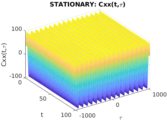
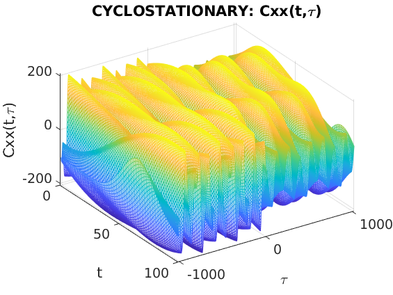
\[\begin{array}{lcl} x(t) & \stackrel{W_T}{\longrightarrow} & \hat{x}_k\\ \bar{x}(t) := E \left[ x(t) \right] & \stackrel{W_T}{\longrightarrow} & \bar{\hat{x}} := E \left[ \hat{x}_k \right]\\ {C_x(t,\tau) := E \left[ x(t) x^{\star}(t+\tau) \right]} & \stackrel{W_T}{\longrightarrow} & {R_{\hat{x}}(l) := E \left[ \hat{x}_k \hat{x}_{k+l}^{\star} \right]}\\ \underbrace{S_x(\alpha,\omega):= \int_0^T \int_{\tau=-\infty}^{\infty} C_x(t,\tau) e^{- j \omega \tau} e^{-j \alpha t} \mathrm{d}\tau \mathrm{d}t}_{Cyclostationary} & \stackrel{W_T}{\longrightarrow} & \underbrace{P_{\hat{x}}(\theta) := \sum_l R_{\hat{x}}(l) e^{-l \theta}}_{Stationary} \end{array}\]

Part II: Nature of dynamics unknown

System identification from output

Is the output cyclostationary?

Distinguish between LTI and Time-Periodic dynamics from data

System identification of time-periodic systems

References

[bamieh1992h2] Bassam Bamieh & Boyd Pearson, The H2 problem for sampled-data systems, Systems & Control Letters, 19(1), 1-12 (1992). link. doi.
[benjamin1954] Benjamin & Ursell, The stability of the plane free surface of a liquid in vertical periodic motion, Proceedings of the Royal Society of London. Series A. Mathematical and Physical Sciences, 225(1163), 505-515 (1954). link. doi.
[Berg_2015] Jordan Berg & Manjula Wickramasinghe, Vibrational control without averaging, Automatica, 58, 72-81 (2015). link. doi.
[craun2015] Mitchel Craun & Bassam Bamieh, Optimal Periodic Control of an Ideal Stirling Engine Model, Journal of Dynamic Systems, Measurement, and Control, 137(7), 071002 (2015). link. doi.
[iwatsubo1974] Iwatsubo, Sugiyama & Ogino, Simple and combination resonances of columns under periodic axial loads, Journal of Sound Vibration, 33, 211-221 (1974).
[kelly1965] Kelly, The stability of an unsteady Kelvin–Helmholtz flow, Journal of Fluid Mechanics, 22(3), 547–560 (1965). link. doi.
[pedlosky2003] Joseph Pedlosky & Jim Thomson, Baroclinic instability of time-dependent currents, Journal of Fluid Mechanics, 490, 189-215 (2003). link. doi.
[poulin2003] Francis Poulin, Flierl & Pedlosky, Parametric instability in oscillatory shear flows, Journal of Fluid Mechanics, 481, 329-353 (2003). link. doi.
[sammarco1997] Paolo Sammarco, Hoang Tran, Oded Gottlieb & Chiang Mei, Subharmonic resonance of Venice gates in waves. Part 2. Sinusoidally modulated incident waves, Journal of Fluid Mechanics, 349, 327-359 (1997). link. doi.
[turner1998] Turner, Miller, Hartwell, MacDonald, Strogatz & Adams, Five parametric resonances in a microelectromechanical system, Nature, 396(6707), 149 (1998).
[vittori1998] Giovanna Vittori, Oscillating Tidal Barriers and Random Waves, Journal of Hydraulic Engineering, 124(4), 406-412 (1998). link. doi.